help("dpois")
dpois(3,0.75)
[1] 0.03321327ppois(2,0.75)[1] 0.9594946Please note that there is a file on Canvas called Getting started with R which may be of some use. This provides details of setting up R and Rstudio on your own computer as well as providing an overview of inputting and importing various data files into R. This should mainly serve as a reminder.
Recall that we can clear the environment using rm(list=ls()) It is advisable to do this before attempting new questions if confusion may arise with variable names etc.
In this example we let \(X\sim \text{Po}(0.75)\) and we calculate \(P(X=3)\) and \(P(X\leq 2)\), and we will plot this distribution.
help("dpois")
dpois(3,0.75)[1] 0.03321327ppois(2,0.75)[1] 0.9594946x<-seq(0,14, length=15)
dx<-dpois(x,0.75)
plot(x,dx, xlab="x value",type="p", ylab="Probability", main="Poisson(0.75) Distribution")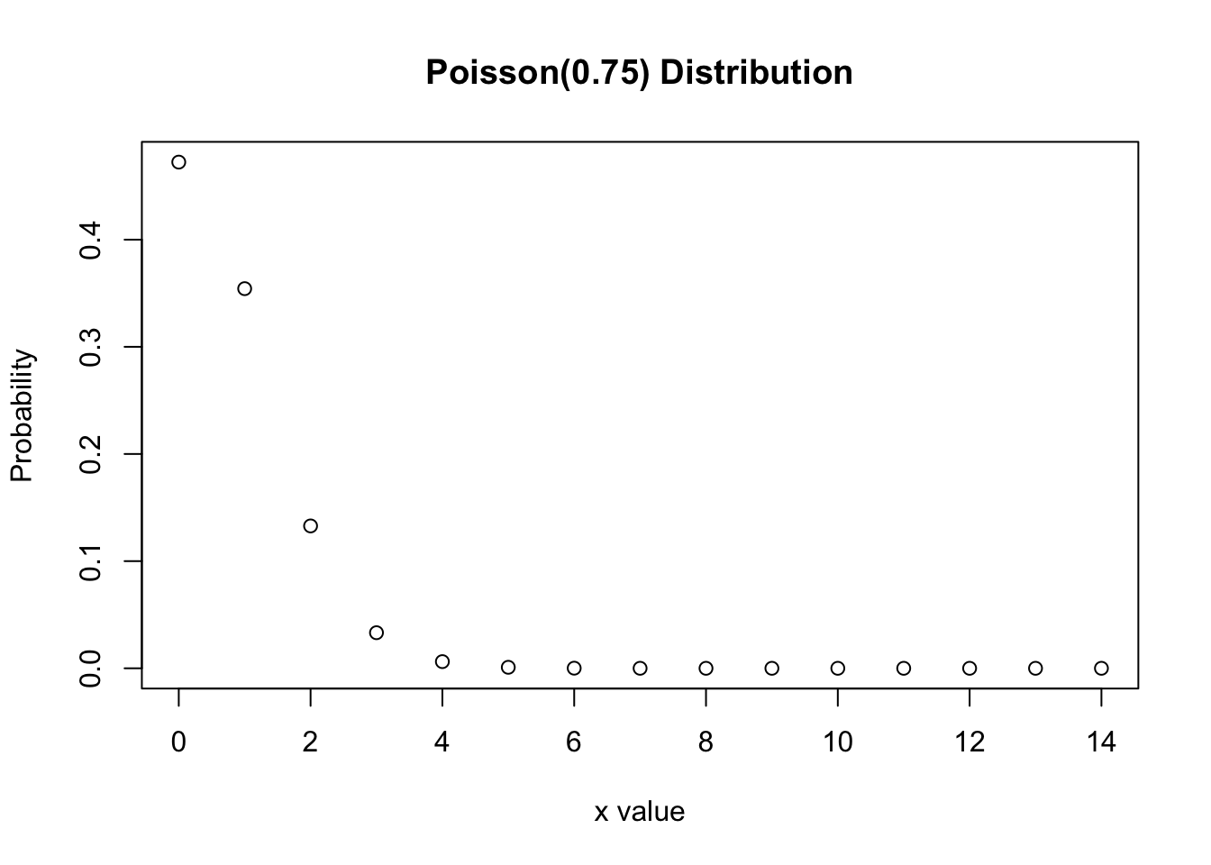
For \(Y\sim Po(1.5)\) find \(P(Y=1)\) and \(P(Y>3)\).
dpois(1,1.5)[1] 0.3346952ppois(3,1.5, lower.tail=F)[1] 0.06564245In this example we will create Poisson random numbers and then test to see whether the numbers generated follow a Poisson distribution.
Note: Everyone’s results will likely be different as this is a random process.
help("rpois")
RandomSample<-rpois(20,2.5)
RandomSample
[1] 2 4 1 1 3 1 7 2 3 5 3 8 3 2 4 0 2 5 2 1mean(RandomSample)[1] 2.95var(RandomSample)[1] 4.260526hist(RandomSample)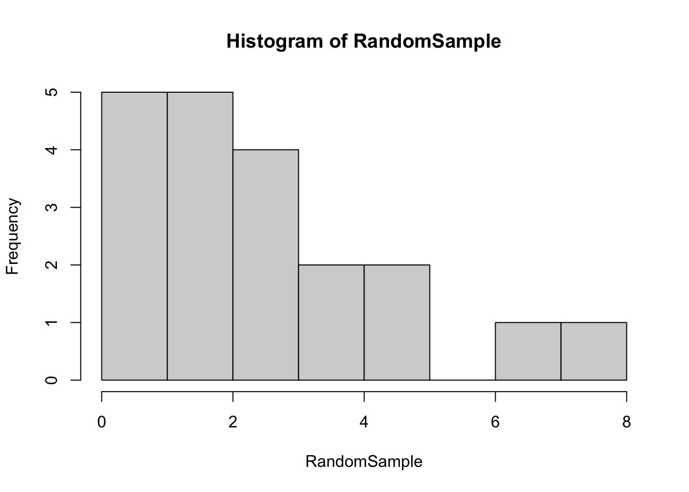
Repeat the example above, but change the mean of the Poisson distribution that you initially generate random numbers from.
This will depend on your individual choice of the mean of the distribution (and the randomness of the procedure).
This example considers creating a log-linear model for count data, i.e. Poisson regression. In the lectures, estimates of the parameters were just stated; now we will use R to obtain these. We will see the full details of the Surgery example and investigate whether Number of Surgery Visits is related to Location via a log-linear model. We assume a Poisson distributed dependent variable and independence.
library(foreign)
Surgery<-read.spss(file.choose(), to.data.frame = T)head(Surgery) Patient Location SurgeryVisits
1 1 0 1
2 2 0 2
3 3 1 5
4 4 1 6
5 5 1 5
6 6 0 1SurgeryPoissonReg<-glm(SurgeryVisits~factor(Location), data=Surgery, family="poisson")
summary(SurgeryPoissonReg)
Call:
glm(formula = SurgeryVisits ~ factor(Location), family = "poisson",
    data = Surgery)

Deviance Residuals:
    Min       1Q   Median       3Q      Max
-1.4138  -0.3379  -0.2238   0.1303   2.0000

Coefficients:
                  Estimate Std. Error z value Pr(>|z|)
(Intercept)         0.8473     0.2673   3.170  0.00152 **
factor(Location)1   0.7033     0.3190   2.205  0.02745 *
---
Signif. codes:  0 '***' 0.001 '**' 0.01 '*' 0.05 '.' 0.1 ' ' 1

(Dispersion parameter for poisson family taken to be 1)

    Null deviance: 14.1586  on 12  degrees of freedom
Residual deviance:  8.9034  on 11  degrees of freedom
AIC: 52.038

Number of Fisher Scoring iterations: 5anova(SurgeryPoissonReg, test="Chisq")Analysis of Deviance Table
Model: poisson, link: log
Response: SurgeryVisits
Terms added sequentially (first to last)
Df Deviance Resid. Df Resid. Dev Pr(>Chi)
NULL 12 14.1586
factor(Location) 1 5.2551 11 8.9034 0.02188 *
---
Signif. codes: 0 '***' 0.001 '**' 0.01 '*' 0.05 '.' 0.1 ' ' 1install.packages("lmtest")library(lmtest)
help("waldtest")
waldtest(SurgeryPoissonReg, test="Chisq")Wald test
Model 1: SurgeryVisits ~ factor(Location)
Model 2: SurgeryVisits ~ 1
Res.Df Df Chisq Pr(>Chisq)
1 11
2 12 -1 4.8621 0.02745 *
---
Signif. codes: 0 '***' 0.001 '**' 0.01 '*' 0.05 '.' 0.1 ' ' 1The Wald Chi-Square statistic is significant for Location (p-value of \(0.027<0.05\)) indicating the significance of the Location variable.
Further, from the earlier output, note that \(\hat{b}_0=0.847\); and \(\hat{b}_1=0.703\), i.e. we have the model, \[ \ln \hat{\lambda}_i=0.847+0.703x_{i1}, \text{ or } \hat{\lambda}_i=e^{0.847+0.703x_{i1}}=e^{0.847}(e^{0.703})^{x_{i1}}. \]
The Poisson Log-linear (PCP Defaults) dataset contains the number of defaults on personal contract plans (PCPs) for a certain car dealership according to their customers’ salary band. The Salary variable has 3 categories, 0, 1 and 2. Create a Poisson log-linear model for these data. You may assume independence and that the dependent variable is Poisson distributed. Make sure you analyse the output.
Hint: In this question the categorical variable (Salary) has more than 2 categories - this makes interpreting the model more complicated. The notes on dummy variables in the lecture notes should help you, along with Example 3 on the R examples class sheet.
library(foreign)
PCP<-read.spss(file.choose(), to.data.frame = T)head(PCP) Customer Salary DefaultNumber
1 1 0 5
2 2 0 6
3 3 1 3
4 4 2 3
5 5 2 5
6 6 1 4attach(PCP)PCPReg<-glm(DefaultNumber~factor(Salary), data=PCP, family="poisson")
summary(PCPReg)
Call:
glm(formula = DefaultNumber ~ factor(Salary), family = "poisson",
    data = PCP)

Deviance Residuals:
    Min       1Q   Median       3Q      Max
-2.1213  -0.2583   0.0000   0.1671   1.5764

Coefficients:
                Estimate Std. Error z value Pr(>|z|)
(Intercept)       1.7228     0.1890   9.116   <2e-16 ***
factor(Salary)1  -0.6242     0.3200  -1.951   0.0511 .
factor(Salary)2  -0.9118     0.3832  -2.380   0.0173 *
---
Signif. codes:  0 '***' 0.001 '**' 0.01 '*' 0.05 '.' 0.1 ' ' 1

(Dispersion parameter for poisson family taken to be 1)

    Null deviance: 16.5487  on 13  degrees of freedom
Residual deviance:  8.9861  on 11  degrees of freedom
AIC: 56.247

Number of Fisher Scoring iterations: 5anova(PCPReg, test="Chisq")Analysis of Deviance Table
Model: poisson, link: log
Response: DefaultNumber
Terms added sequentially (first to last)
Df Deviance Resid. Df Resid. Dev Pr(>Chi)
NULL 13 16.5487
factor(Salary) 2 7.5627 11 8.9861 0.02279 *
---
Signif. codes: 0 '***' 0.001 '**' 0.01 '*' 0.05 '.' 0.1 ' ' 1install.packages("lmtest")library(lmtest)
waldtest(PCPReg, test="Chisq")Wald test
Model 1: DefaultNumber ~ factor(Salary)
Model 2: DefaultNumber ~ 1
Res.Df Df Chisq Pr(>Chisq)
1 11
2 13 -2 7.3907 0.02484 *
---
Signif. codes: 0 '***' 0.001 '**' 0.01 '*' 0.05 '.' 0.1 ' ' 1Analysis of the output:
The deviance/df is 0.817, indicating a good model fit. Furthermore, the Wald chi-square statistic is significant indicating the significance of the Salary variable.
The three categorical variables are combined into 2 dummy variables, say \(d_1\) and \(d_2\), where \(d_1\) and \(d_2\) take the values \(0\) or \(1\), i.e. we have a model of the form: \[ y_i=e^{b_0+c_{1}d_{1}+c_{2}d_{2}}. \]
In particular, we have: \[ y_i=e^{1.723-0.912d_{1}-0.624d_{2}}. \]
The base case is where \(d_1=d_2=0\), and this corresponds to salary band \(0\) in this case. Therefore, for salary band 0, we have, \[ y_i=e^{1.723}=5.6, \quad \text{i.e. 5.6 defaults for people in band $0$.} \]
Another possibility is when \(d_1=1\) and \(d_2=0\), and this corresponds to salary band \(2\). In this case the model is, \[ y_i=e^{1.723-0.912\times1-0.624\times 0}=2.25, \quad \text{i.e. 2.25 defaults for people in band $2$.} \]
Finally, for \(d_1=0\) and \(d_2=1\), i.e. for salary band \(1\), we have, \[ y_i=e^{1.723-0.912\times0-0.624\times 1}=3, \quad \text{i.e. 3 defaults for people in band $1$.} \]